The TomTom Maps SDK for Web offers the easiest way to access the TomTom APIs for displaying maps and geo information, and is easy to interact with regardless of your coding experience level. The SDK is completely framework-agnostic and can be used to leverage not only the TomTom APIs, but also data coming from any other API.
In this article we explore a potential use case for showing multiple layers with the TomTom Maps SDK: We’ll build a map that displays the population density of the USA in the form of a heatmap. A heatmap enables map viewers to perceive the population density of points independently of the zoom factor. It’s the least constrained of all display styles, because it doesn’t correspond to geographic boundaries. Other options for display styles include dot density, choropleth, and hexagonal binning.
Project Preparation
Here’s what we need to build our custom map view:
- An API key for accessing the TomTom API
- The TomTom Maps SDK
- Some population density data
To obtain an API key, start by registering as a developer on the TomTom developer portal. This will give you a sample API key you can use later to access all other TomTom APIs in the future..
After registering successfully, you can also download the latest version of the TomTom Maps SDK for Web. For this article, we’ll actually just reference the necessary files from an online location, so that is all you will need to download!
The population density data can be retrieved from the U.S. Census Bureau, but we’ll use a premade GeoJSON file that contains the density values from this Wikipedia article. The data was prepared by Mike Bostock.
Building the Map Display
- An HTML file where we put everything together.
- References to the TomTom SDK files (CSS and JavaScript).
- Some code to initialize the map on the HTML document.
To get going, open your text editor and start a simple HTML file. Since we can take the TomTom Web SDK files from the available content delivery network (CDN), we don’t have to download anything.
All in all, the boilerplate to display a map is minimal. We’ll just introduce some custom CSS to obtain a full-screen map display, only for convenience.
The code in action looks like this:
					<link rel="stylesheet" href="https://api.tomtom.com/maps-sdk-for-web/cdn/5.x/5.36.1/maps/maps.css">
<style>
html, body {
  padding: 0;
  margin: 0;
  width: 100%;
  height: 100%;
}
body {
  display: flex;
  flex-direction: row;
}
#map {
  flex: 1;
  height: 100%;
  width: 100%;
}
</style>
<div id="map"></div>
<script src="https://api.tomtom.com/maps-sdk-for-web/cdn/5.x/5.36.1/maps/maps-web.min.js"></script>
<script>
tt.map({
  container: document.querySelector('#map'),
  key: 'your-api-key',
  language: 'en-GB',
  center: [-96.7098725, 39.0640021],
  zoom: 4,
});
</script>
Notably, we set the language explicitly to British English. The map should be centered at some location in the United States, with the zoom being configured such that most parts of North America are visible on desktop resolutions.
Obtaining the Heatmap Data
With the map correctly displayed, we can go on to display the desired heatmap layer. First, however, we need to obtain the required data. Since the data is already available in a JSON file, we only need to fetch the file’s content from the server. Ideally, this can be done using the fetch API. For older browsers, we might need to support different ways of obtaining the contents of a JSON file.
Assuming that the file is called us-states.json, we can retrieve it with the following code:
					fetch('./us-states.json')
  .then(res => res.json())
  .then(data => {
	// ...
  })
  .catch(err => {
      // ...
  });
Fetching a resource from the network is an asynchronous process. Thus, we get back a Promise, which we can use to inspect the response. For production-ready code we should also take care of the catch clause. In the simple example above, we perform the same error handling in any case, as a simple “catch’em all” construct is sufficient.
Once we interpret the body of the raw response as JSON, we obtain another Promise, which leads to the callback where we use the data argument. We already know that the data argument will be a correctly formatted GeoJSON object. We can use this information to build a new layer for our map.
Density Heatmap Layer
With the data in place, we need to look at how to actually integrate a map layer. Luckily, a functional example already exists. Still, in addition to the information from that example and the official documentation, it’s nice to know what’s really going on under the hood.
The TomTom Maps SDK for Web is not a completely new product but rather a combination of successful open-source libraries with a commercial map-display engine to access TomTom’s proprietary API. While the map-related information is all coming from the API, the view completely relies on these libraries. In addition, the TomTom Maps SDK has a small facade on top to make working with all these layers seamless and efficient. Furthermore, it provides the right access point to the TomTom API—all we need to do is to supply our API key as shown in the first code snippet.
Now, for adding layers, we’ll use the addLayer API, which will interact with a portion of the SDK supported by the open source Mapbox GL JS.
Basically, all we need to do is call addLayer once the map has finished loading. There are three options that are of interest to us:
- id — remove or update the layer
- source — configure the layer’s data source
- type — set to heatmap to display the population density in the form of a heatmap
And here they are in action:
					map.addLayer({
  id: 'density',
  source: {
	type: 'geojson',
	data,
  },
  type: 'heatmap',
});
The heatmap layer can also be configured using additional paint options, which include the colors to use, the kind of heatmap, and its shape. The most important setting for painting the density is heatmap-weight. This option helps to define the value for drawing the heatmap. While a linear scale may be a good beginning, we’ll soon find out that it’s not ideal for displaying the relevant information.
Another issue is that the US states are actually defined as multi-polygons, that is, multiple groups of points. While some states (such as Texas) can be well described by a single polygon with points at all corners, other states (like Hawaii) require multiple polygons. Usually, these groups represent different islands.
The issue with using multiple points is that each point is used to display the heatmap, which means we need to define the geometry as a whole. Let’s try to bring it all together!
Bringing Everything Together
With the given data, there are obvious choices we won’t follow. One possibility could be to reduce the states to a single point (in the center of the state), such that each density point reflects just one state. Another idea might be to use a different type of layer, such as a choropleth, to illustrate the states with a given color. What we are after, however, is a heatmap.
Let’s play around with the properties, most notably the radius and weight of the heatmap. Obviously, the weight of the heatmap points is quite important and should be adjusted to the density given in the GeoJSON. Using an exponential weight also seems natural; we only need to determine the scale.
The following snippet sets the heatmap weight according to the density property in the GeoJSON data. It also uses an exponential scale that puts values from 1 to 10000 into the 0 to 1 range.
					{
  "type": "exponential",
  "property": "density",
  "stops": [
	[1, 0],
	[10000, 1]
  ]
}
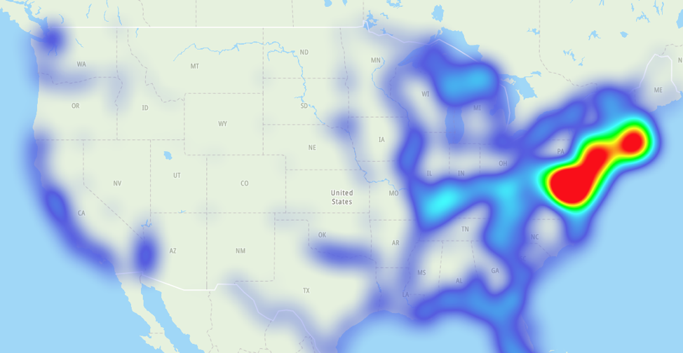
For the radius we can go wild. We can adjust the radius with the zoom level or keep it constant. We’ll start with a constant of 50. Let’s see how it looks:


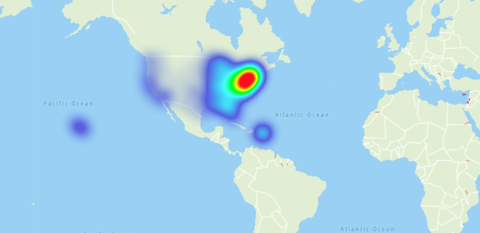
This looks decent at the given zoom level, but becomes inaccurate very quickly. Luckily, we can use a zoom-specific version that counters such problems:
					[
  "interpolate",
  ["linear"],
  ["zoom"],
  0, 10,
  9, 80,
]
As a result, even with maximum zoom out, we can identity the increasing population density on the coasts, especially the East Coast.


Finally, the full JavaScript code to get this working remains quite minimal:
					const container = document.querySelector('#map');
const map = tt.map({
  container,
  key: 'your-api-key',
  language: 'en-GB',
  center: [-96.7098725, 39.0640021],
  zoom: 4,
});

fetch('./us-states.json')
  .then(res => res.json())
  .then(data => {
	map.addLayer({
  	id: 'density',
  	source: {
    	type: 'geojson',
    	data,
  	},
  	type: 'heatmap',
  	paint: {
    	'heatmap-radius': [
      	"interpolate",
      	["linear"],
      	["zoom"],
      	0, 20,
      	9, 80,
    	],
    	'heatmap-weight': {
      	type: 'exponential',
      	property: 'density',
      	stops: [
        	[1, 0],
        	[10000, 1],
      	],
    	},
  	},
	});
  })
  .catch(err => {
	console.error(err);
  });
Conclusion
Using the TomTom Maps SDK for Web with custom map information is straightforward and approachable for developers of any level. Multiple options and countless examples provide enough help to let us get started efficiently. In this article, we showed how to present population density data in the form of a heatmap layer. What will you build?
This post was originally posted on TomTom’s blog.
If you’re interested in developing expert technical content that performs, let’s have a conversation today.


