In the first article of this series, we learned what hyperparameter tuning is , its importance, and our various options. In this hands-on article, we’ll explore a practical case to explain how to tune hyperparameters on XGBoost. You just need to know some Python to follow along, and we’ll show you how to easily deploy machine learning models then optimize their performance.
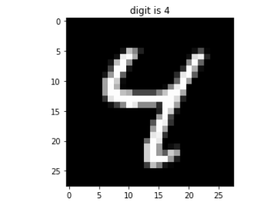
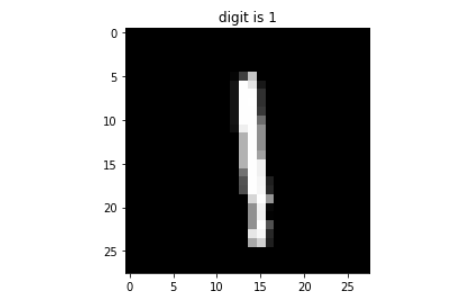
We’ll use the Modified National Institute of Standards and Technology (MNIST) database, including 60,000 training samples and 10,000 test samples. Each sample is an image of a handwritten digit, normalized to a 28 by 28-pixel box and anti-aliased (grayscale levels).
The figures below are a couple of samples from the MNIST database:
To build our digit identification model, we’ll use the popular library, XGBoost. Then to tune it, we will use the scikit-learn library, which provides a relatively easy and uniform hyperparameter tuning method. Let’s get started.
Pre-processing the original MNIST files
First, we download the four files in the MNIST data set: train-images-idx3-ubyte and train-labels-idx1-ubyte for the training, and t10k-images-idx3-ubyte and t10k-labels-idx1-ubyte for the test data.
Then, we convert the ubyte files to comma-separated values (CSV) files to input them into the machine learning algorithm.
The function below performs the conversion:
					def convert(imgf, labelf, outf, n):
    f = open(imgf, "rb")
    o = open(outf, "w")
    l = open(labelf, "rb")

    f.read(16)
    l.read(8)
    images = []

    for i in range(n):
      image = [ord(l.read(1))]
      for j in range(28*28):
        image.append(ord(f.read(1)))
        images.append(image)

    for image in images:
      o.write(",".join(str(pix) for pix in image)+"\n")

    f.close()
    o.close()
    l.close()

convert("train-images-idx3-ubyte",
        "train-labels-idx1-ubyte",
        "mnist_train.csv", 60000)
convert("t10k-images-idx3-ubyte",
        "t10k-labels-idx1-ubyte",
        "mnist_test.csv", 10000)
Now we need to adjust the label column for the machine learning algorithm. The training set is in column 5, while the test set is in column 7. We need to rename those columns and generate new CSV files.
					import pandas as pd

# read the converted files
df_orig_train = pd.read_csv('mnist_train.csv')
df_orig_test = pd.read_csv('mnist_test.csv')

# rename columns
df_orig_train.rename(columns={'5':'label'}, inplace=True)
df_orig_test.rename(columns={'7':'label'}, inplace=True)

# write final version of the csv files
df_orig_train.to_csv('mnist_train_final.csv', index=False)
df_orig_test.to_csv('mnist_test_final.csv', index=False)
We have now finished pre-processing the data set and can start building the model.
Building model parameters without tuning hyperparameters
Let’s start by building the model without any hyperparameter tuning. Instead, we will use typically recommended values for our hyperparameters.
To run this code yourself, you’ll need to install NumPy, sklearn (scikit-learn), pandas, and XGBoost using pip, Conda, or another Python package management tool. Note that this isn’t intended to be a comprehensive XGBoost tutorial. If you’re new to XGBoost, we recommend starting with the guides and tutorials in the XGBoost documentation.
First, we’ll define a model_mnist function that takes a hyperparameter list as input. This makes it easy to quickly recreate the model with different hyperparameters.
Also, for practical reasons, we will work with the first 1,000 samples from the training dataset. The MNIST training dataset has 60,000 samples with high dimensionality (784 features), which means about 47 million data points. Building the model for the complete dataset takes time (in the range of 10-15 minutes for an 8-core CPU), so it will take many hours, or even days, to perform hyperparameter tuning on a single machine. So, using a smaller dataset while we’re learning allows us to experiment with different tuning techniques more quickly.
					import numpy as np
import pandas as pd   # data processing, CSV file I/O (e.g. pd.read_csv)
import xgboost as xgb
from sklearn.model_selection import train_test_split
from sklearn import metrics

def model_mnist(params):

    # Input data files are available in the "./data/" directory.
    train_df = pd.read_csv("./data/mnist_train_final.csv")
    test_df = pd.read_csv("./data/mnist_test_final.csv")

    # limit the dataset size to 1000 samples
    dataset_size = 1000
    train_df = train_df.iloc[0:dataset_size, :]
    test_df = test_df.iloc[0:dataset_size, :]

    y = train_df.label.values
    X = train_df.drop('label', axis=1).values

    # build train and validation datasets
    X_train, X_val, y_train, y_val = train_test_split(X, y, test_size=0.15)
    print("Shapes - X_train: ", X_train.shape,
          ", X_val: ", X_val.shape, ", y_train: ",
          y_train.shape, ", y_val: ", y_val.shape)

    train_data = xgb.DMatrix(X_train, label=y_train)
    val_data = xgb.DMatrix(X_val, label=y_val)

    n_rounds = 600
    early_stopping = 50

    # build the model
    results = {}

    model = xgb.train(params,
                      train_data,
                      num_boost_round=100,
                      evals=[(val_data, 'val')],
                      evals_result=results)

    # let’s check how good the model is
    x_test = test_df.drop('label', axis=1).values
    test_labels = test_df.label.values
    test_data = xgb.DMatrix(x_test)

    predictions = model.predict(test_data)

    accuracy = metrics.accuracy_score(test_labels, predictions)

    return accuracy


if __name__ == '__main__':

    # define number of classes = 10 (digits)
    # and the metric as merror (multi-class error classification rate)
    default_params = [
        ("num_class", 10), ("eval_metric", "merror")
    ]

    accuracy_result = model_mnist(default_params)

    print("accuracy: ", accuracy_result)
Save the above Python code in a .py file (for instance, mnist_model.py) and run it from the command line:
$ python mnist_model.py
We should see the following output:
					Shapes - X_train:  (850, 784) , X_val:  (150, 784) , y_train:  (850,) , y_val:  (150,)
[0]	val-merror:0.326667
[1]	val-merror:0.233333
 .
 .
[98]	val-merror:0.166667
[99]	val-merror:0.166667
accuracy:  0.826
The output shows we obtained an accuracy of 82.6 percent (that is, our model correctly classified 82.6 percent of test samples).
Tuning hyperparameters
Now we’ll tune our hyperparameters using the random search method. For that, we’ll use the sklearn library, which provides a function specifically for this purpose: RandomizedSearchCV.
First, we save the Python code below in a .py file (for instance, random_search.py).
					import numpy as np
import pandas as pd
import xgboost as xgb

from sklearn.model_selection import train_test_split
from sklearn.model_selection import RandomizedSearchCV

def random_search_tuning():
    # Input data files are available in the "./data/" directory.
    train_df = pd.read_csv("./data/mnist_train_final.csv")
    test_df = pd.read_csv("./data/mnist_test_final.csv")
    print (train_df.shape, test_df.shape)

    y = train_df.label.values
    x = train_df.drop('label', axis=1).values

    # define the train set and test set
    x_train, x_val, y_train, y_val = train_test_split(x, y, test_size=0.05)
    print("Shapes - X_train: ", x_train.shape,
          ", X_val: ", x_val.shape, ", y_train: ",
          y_train.shape, ", y_val: ", y_val.shape)

    params = {'max_depth': [3, 6, 10, 15],
              'learning_rate': [0.01, 0.1, 0.2, 0.3, 0.4],
              'subsample': np.arange(0.5, 1.0, 0.1),
              'colsample_bytree': np.arange(0.5, 1.0, 0.1),
              'colsample_bylevel': np.arange(0.5, 1.0, 0.1),
              'n_estimators': [100, 250, 500, 750],
              'num_class': [10]
              }

    xgbclf = xgb.XGBClassifier(objective="multi:softmax", tree_method='hist')
    clf = RandomizedSearchCV(estimator=xgbclf,
                             param_distributions=params,
                             scoring='accuracy',
                             n_iter=25,
                             n_jobs=4,
                             verbose=1)

    clf.fit(x_train, y_train)

    best_combination = clf.best_params_

    return best_combination


if __name__ == '__main__':

    best_params = random_search_tuning()

    print("Best hyperparameter combination: ", best_params)
Our expected output looks something like this:
					Fitting 5 folds for each of 25 candidates, totaling 125 fits
Accuracy:  0.858
Best hyperparameter combination:  {'subsample': 0.9,
                                   'num_class': 10,
                                   'n_estimators': 500,
                                   'max_depth': 10,
                                   'learning_rate': 0.1,
                                   'colsample_bytree': 0.6,
                                   'colsample_bylevel': 0.7}
The accuracy has improved to 85.8 percent. We’ve now found the best hyperparameter combination for our model.
Next steps
After running our untuned and tuned models, we discovered that our model with tuned hyperparameters has better accuracy. The tuned model can make better predictions on new data, so it can more accurately identify images of digits beyond those in the training set.
In the final article of our three-part series, we’ll explore hands-on how distributed hyperparameter tuning improves our results even more. We’ll use Ray to deploy our Python machine learning model to the cloud for distributed tuning using Ray Tune.
If you’re interested in developing expert technical content that performs, let’s have a conversation today.